Financial Statement projections – beyond numbers to accounting concepts and their relationships
Using data, extracted from published corporate results, Exerica automatically builds models for financial statements. These include Income statements, Balance sheets, and Cash flows, amongst many others. Where we have deployed the model for several years, we can use it to project the next reporting period.
We have previously developed the regression model for financial time series projections, which presented good results for individual time series. Taking this as a basis, we commenced the forecasting of entire financial statements, which I will discuss in this article using, the Income statement as an example.
But data in Exerica is presented not just as individual financial indicators or even time series of these. These time series, and specific number values also reflect mathematical relationships describing the accounting structure. And the algorithm we have developed allows us to project an entire financial statement while preserving the integrity of the accounting structure and the relationships between the constituent parameters of the accounting structure.
The Current Cutting Edge of Forecasting
Forecasting company financials is an integral part of corporate risk management at any financial institution. There are numerous publications presenting different approaches on the subject (1, 2, 3, 4, 5). In addition to this , research teams of investment banks, funds and investment companies certainly also have their own proprietary forecasting models, which they do not publish.
Machine learning is commonly used to generate such models. To forecast financial time series, two classes of ML-models are mainly used:
- Autoregressive models
- Neural networks
An Autoregressive model would calculate a predicted value based on one or more previous values of the time series, as well as external (exogenous) variables, which usually include macroeconomic data. The type of dependency and the depth of regression are the hyperparameters of the model. The coefficients at the previous values of the time series, as well as at the external variable are the parameters of the model estimated by the supervised learning process. When developing a regression model, we can specify dependencies determined by the properties of the domain (eg, seasonality). Due to the relatively small number of parameters, аutoregressive models could be trained on low-frequency time series.
Neural network models calculate the predicted value as the output of the neural network. The hyperparameters of the model are, in particular, the architecture of the neural network and the number of neurons in the layers. Neural network models are commonly used to forecast high-frequency time series, such as stock prices, for which a large amount of historical data is available. Use of these models is limited by a lack of training data volumes, which can mean the resulting models are insufficiently “smart” when it comes to, identifying complex dependencies in financial statements.
The biggest challenge for the existing models, however, is forecasting any company accounting structure as a whole. That is, projecting separate elements of company accounts in such a way that they all remain related to each other mathematically and analytically (for example Net profit remains the sum of Pre-tax Profit and Income tax, Gross profit remains equal to the difference between Revenue and Cost of Sales etc.). We believe that no existing model is able to address this problem, and this has a lot to do with the fact that the training data (provided by the major data providers such as Bloomberg, Refinitiv, Capital IQ) is not analytically consistent in the first place.
Our forecasting models take advantage of Exerica’s ability to identify and extract the entire structure of a company’s accounts, which takes data integrity to a whole new level. This enables us to forecast company performance as whole rather than in pieces which are difficult to relate to a whole.
Exerica’s Financial statement projection algorithm
Exerica’s projection model for financial statements uses the autoregressive approach. To describe the projection algorithm we have developed I would start with the projection of an Income Statement.
We could look at a financial statement as an n-dimensional time series:
\(X_t=(x_{t1},…,x_{tn})\)
Since we are considering the financial statement, the components of this vector are not independent. For example, the Operating profit can be represented as the sum of Revenue and Total Costs. In general, this mathematical consistency of a financial statement can be written as a linear relationship:
\(M \cdot X_t = 0\), where \(M=(m_{ij})\) is square matrix (time independent) and any \(m_{ij} =\{-1,0,1\}\)
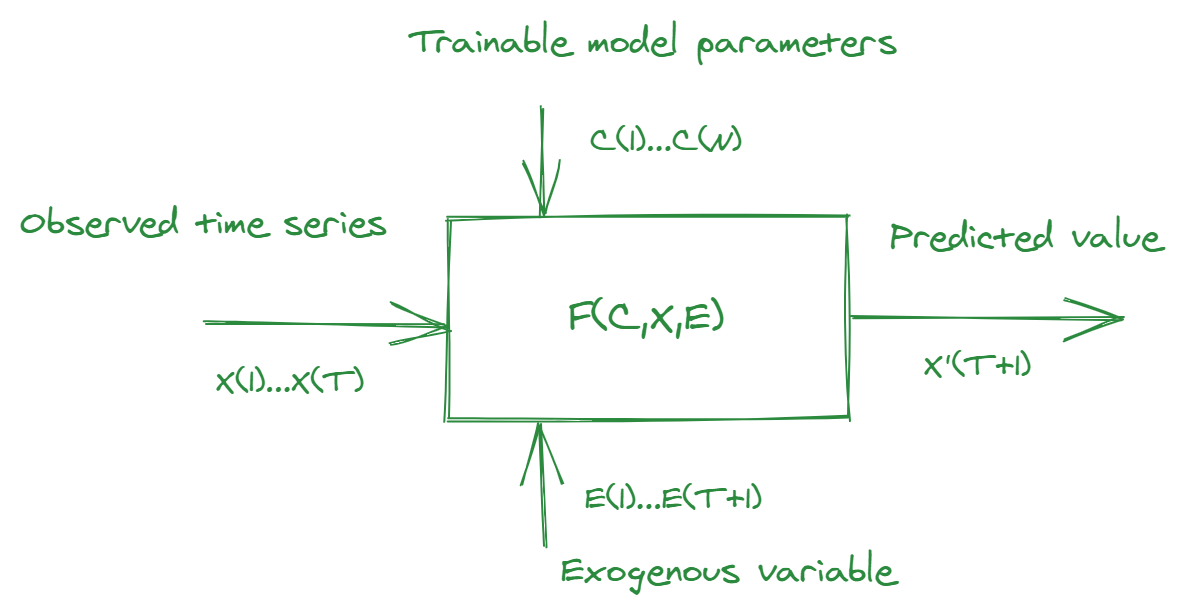
Given a time series for period \({1,…,T}\) we would consider the projection algorithm as a function:
\(X’_{T+1}=F(C_1,…,C_N, X_1,…,X_T, E_1,…,E_{T+1})\)
with constraint \(M \cdot X’_{T+1}=0\)
where \(C_1,…,C_N\) are model parameters and \(E_1,…,E_{T+1}\) are exogenous variable values (optional).
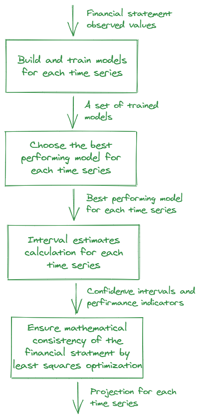
Based on our autoregressive approach to predicting individual indicators, we have developed the following algorithm:
- Considering the frequency of the time series a set of the k models would be chosen.
- For each indicator from a financial statement each of the k models is trained on the set of observations \(x_{0i},…,x_{Ti}\). As the result of this stage, a set of trained models would be built: \(r_{ij}, i=\{0,…,n\}, j=\{1,…,k\}\).
- A competition between the trained models is held: backtesting is carried out for each of the models. The best performing model for each indicator would be chosen for the next stage.
- The chosen models are used to calculate interval estimates \([x_{(T+1)i}^l, x_{(T+1)i}^u]\) as the confidence interval for prediction.
- To ensure the mathematical consistency of the financial statement’s accounting structure, projected values are adjusted. This adjustment could be written as an optimization problem with constraints:
\(
\min\limits_{
\small
\begin{matrix}
x_i\in [x_{(T+1)i}^l, x_{(T+1)i}^u] \\
i \in \{1,..,n\}
\end{matrix}
} M \cdot
\begin{pmatrix}
x_1\\
…\\
x_n
\end{pmatrix} = 0
\)
The problem is solved by the least squares method. - Considering the quality indicators of backtesting, the size of confidence intervals and some additional parameters, the confidence level for each indicator from financial statement is calculated.
As a result we would have the vector of projected values \(X’_{T+1}\) with \(M \cdot X’_{T+1} \approx 0\).
Real-time regression model competition
The stages 1-3 of the algorithm are completed by competition between the trained autoregressive models. These stages are quite important as they determine the model that best takes into account external factors affecting a particular time series. First, we select a set of models for training. This set is formed from various combinations of the following regression models:
- Auto-Regressive (AR)
- Moving Average (MA)
- Auto-Regressive Moving Average (ARMA)
- Auto-Regressive Integrated Moving Average (ARIMA)
- Seasonal Auto-Regressive Integrated Moving Average (SARIMA)
We also take exogenous variables into account, including those which could be correlated with projected indicators. For example they could be: national currency exchange rate for the country a company operates in, commodity prices affecting inputs, industry or stock indexes (Eg, SPX for US companies).
We’ve also introduced another improvement to refine the forecast accuracy of a number of financial statement indicators. We consider the time series of indicators, as well as their ratios, and choose the best performing one. For example we are projecting OPEX divided by Revenue to estimate the forecasted OPEX.
As a result we would choose the model that performs best (least errors) in the backtesting process. At the same time, the most significant variable factors and external variables from the set under consideration are automatically selected.
The overall model evaluation process including ML, model competition, optimization and projection calculation usually takes from 10 to 20 seconds on a common PC, and does not require specific computing resources such as GPUs. This makes it possible to run the process on demand and to cache the results with one operation of the process.
Example
For example let’s look at several companies’ latest fillings for 1Q 2021 and compare their revenue projections against the reported as well as consensus estimates.
| Ticker | Projected | Reported | Consensus |
|---|---|---|---|
| $CVS | 69.5bn | 69.1bn | 68.4bn |
| $GOLD | 2.9bn * | 2.95bn | 3.01bn |
| $RNG | 349.6m ** | 352.4m | 339.9m |
| $SRE | 3.16bn | 3.26bn | 3.25bn |
* – The algorithm determined the relationship of the indicator with the commodity (gold) price, which influenced a reduction of the estimate and resulted in a more accurate estimate than the consensus forecast of analysts.
** – The algorithm determined the relationship of the indicator with the S&P500 index, which influenced a smaller reduction of the estimate and resulted in a more accurate estimate than the consensus forecast of analysts.
In Conclusion
We developed a competition-based multi-model projection tool for online financial statement analysis. The key features of our tool are:
- Use of a number of regression models to determine the best performing one
- Projection of the whole accounting structure, preserving arithmetic relations
- Consideration of internal parameter ratios
- Consideration of external factors: currency exchange rates, stock and commodity indices
- Rapid projection model evaluation: 20-30 seconds for a company financial statement.
We assessed the performance of our projection algorithm during 1Q 2021 reporting period. As we can see it’s accuracy is comparable with consensus analyst estimates. Sometimes our model outperforms consensus analyst estimates when our algorithm automatically determines the key relationship factor.