Projecting time series with soft real-time machine learning
At Exerica we collect numerical data extracted from corporate reports as a consistent time series. That means we accumulate a lot of data that goes beyond ordinary statements and earnings data, and a lot which goes beyond ‘financial’ subsets.
As an example we can identify how much ImmunoGen has spent on clinical and preclinical testing for each quarter for the last six years (here). An issue faced by all analysis, and therefore one we need to address, is the ability to forecast or project time series into the future.
We first looked at deep learning with recurrent neural networks, such as LSTM (long-short term memory), or combinations of convolution networks. These are the standard approaches to addressing data projection, and there are a number of solutions for time series forecasting with neural networks (insert links here). But they all cover only a situation where the time series is “high frequency” and contains hundreds of data points. The data we address at Exerica is generally not so high frequency, so we looked at regression models – the other “common” set of forecasting models.
As the data Exerica works most commonly with comes from periodically published corporate
reports or statements, we see that most of the time series we need to work with are non-stationary. We can distinguish the following major time series components:
- Trend – linear increasing or decreasing
- Nonlinear dependency on previous values, including, but not limited to, seasonality
- External and unrevealed factors (which could be considered as random variables)
The model description
For modeling and forecasting of non-stationary time series the ARIMA model class is widely used (Auto-Regressive Integrated Moving Average). Assuming that the time series being addressed is differentially stationary (i.e. its differences are stationary) we can use auto regressive moving average models for time series differences. This model also can utilise a seasonal component in a linear and non-linear way.
Given a time series \(X_t\) the \(ARIMA(p,d,q)\) modeled process can be written as:
\(\triangle^dX_t=c+\sum_{i=1}^p a_i \triangle^dX_{t-i} + \sum_{i=1}^q b_i\epsilon_{t-i} + \epsilon_t\)where \(c\) is an intercept, \(\triangle\) is the first-difference operator and we assume that \(\epsilon_{t} \sim N(0, \sigma^2)\). Equivalently the model can be written as:
\(a_p(L)\triangle^d X_t = c + b_q(L) \epsilon_t\)where:
\(a_p(L) = 1 – \sum_{i=1}^p a_i L^i\) is autoregressive lag polynomial,
\(b_q(L) = 1 + \sum_{i=1}^p b_i L^i\) is moving average lag polynomial
and \(L\) is the lag operator.
With the above we can model only incorporate additive seasonal effects by including specific lags to the model. For example, to model year-over-year effects we would add dependency on the 4th moving average lag.
To model a multiplicative seasonal effect we can adjust the model to \(ARIMA(p,d,q)\times(P,D,Q)_s\), where the uppercase letters indicate the parameters of the seasonal component and \(s\) is the periodicity of the seasons (for example, 4 yearly periods for quarterly data). The process can be written as:
\(a_p(L)\widetilde{a}_P(L) \triangle^d\triangle_s^D X_t = A(t) + b_q(L) \widetilde{b}_Q(L^s) \epsilon_t\)where:
\(a_p(L)\) is the non-seasonal autoregressive lag polynomial,
\(b_q(L)\) is the non-seasonal moving average lag polynomial,
\(\widetilde{a}_P(L)\) is the seasonal autoregressive lag polynomial,
\(\widetilde{b}_Q(L)\) is the seasonal moving average lag polynomial,
\(A(t)\) is the trend polynomial.
We also assume a need to to add an exogenous variable to the model, so the model in general can be specified as:
\(X_t = \beta_tY_t + U_t\\a_p(L)\widetilde{a}_P(L) \triangle^d\triangle_s^D U_t = A(t) + b_q(L) \widetilde{b}_Q(L^s) \epsilon_t\)
where \(Y_t\) is the exogenous process.
Given the general model \(ARIMA(p,d,q)\times(P,D,Q)_s\) we would consider \(p, d, q, P, D, Q\) and \(s\) the hyperparameters of our model. To produce a predictive model we use machine learning techniques to estimate the coefficients of the lag and trend polynomials for the selected hyperparameters. The common estimation technique we would use for this is maximum likelihood estimation (MLE).
Model tuning and parameter estimation
We performed a number of statistical tests and model quality assurance tests on sample datasets from our database to select hyperparameters for the model. We used the following metrics to estimate the quality of the hyperparameters:
- The mean absolute percentage error (MAPE) for the last estimated year
- The absolute percentage error (APE) of one-step forecast
- The 0.9-quantile for the absolute percentage error of one-step forecast
- The ratio of time series for which the model is converged
We consider the model converged if, and only if, the MLE process is converged and the last-year MAPE is below the given threshold. We tuned the hyperparameters to bring those metrics to acceptable ranges. On our sample dataset we get following metrics:
| Converged ratio | 82% |
| Average MAPE | 9,4% |
| Average 1-step APE | 18% |
| APE 0.9-quantile | 46% |
Currency exchange rates were considered a key exogenous variable. We tested the dependence hypothesis of some headline numbers (“Revenue” and related time series) for companies from our database with the exchange rate the company reports in by using a time series model as mentioned above, and comparing the metrics produced against the metrics for the model without exogenous variables. The tests on our sample dataset covering companies with 10 different currencies showed no significant model quality dependency on currency exchange rates. But we do see some degradation of the model with exogenous variables – the ratio of converged models drops to 76%.
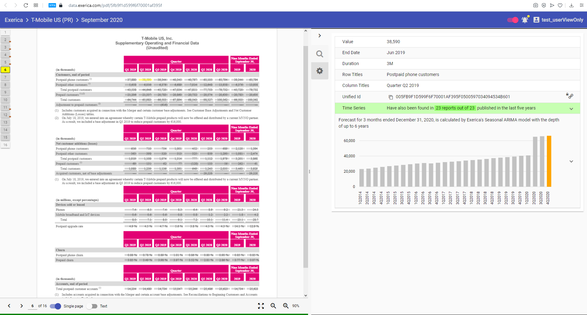
Projections implementation with Exerica
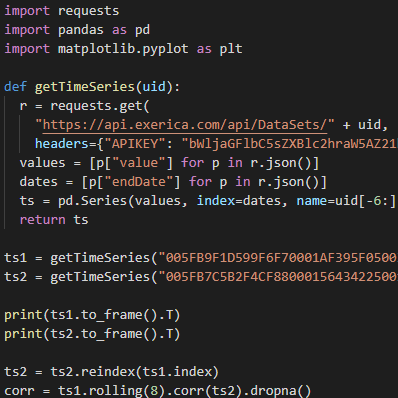
As mentioned above we want to forecast any of the time series in our database. Currently (Jan 2021) the Exerica database contains about 5.5 million time series – of different types with different characteristics. So the parameters of different time series models would vary. Our approach to solving this problem is to estimate the model parameters and to calculate the forecast for the time series in real-time as it is requested by the user. We have implemented this solution in our analytical service by utilizing the power of Python and statsmodels library. The estimation and the prediction processes both take less than a second on our hardware with only a single-CPU consumption. This meets the requirement for soft real-time calculation and data visualisation in a web application. The forecast for any given time series is visualized in the Exerica web application on the time series bar chart (as you can see on screenshot below).